Front-Loading of Flux Control

Originally Posted on December 20, 2019 by hsauro

There is an interesting property that straight chain pathways have which I call front-loading. The phenomenon has been known for some time and I describe it in detail in my recent textbook on Metabolic Control Analysis. Let’s say we have a straight chain of reactions, something like:

  

There are no long-range feedback loops (other than short-range product inhibition) and it is assumed that for a given reaction, increases in substrate cause the reaction rate to increase and increases in the product causes the reaction to decrease. Each reaction is reversible using a simple reversible mass-action rate law: . I assume that  and  are fixed species. Given suitable rate constants and equilibrium connstants for each reaction, the system will admit a steady state. A question to ask is what is the distribution of flux control across the chain? There are two ways to answer this, we can use theory, this gives us what the distribution is and insight into why or we can do simulation but this will just tell us what the distribution is likely to be. For now let’s do a simulation.

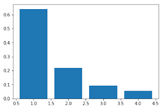
The code is shown below. The code defines a four-step straight-chain, runs 10,000 simulations, randomizing the rate constants for each simulation. Each time it does a simulation we compute the flux control at each step, store this information and then at the end, plot histograms of the distribution of the flux control coefficients. Scroll down to see the plots. The average values for the flux control coefficients is shown in the histogram:

The distribution of flux control is shown below. The vertical axis is the frequency and the x-axis the value of the flux control coefficient from zero to 1.0. The red curve corresponds to the flux control for the first step, on average this has the highest control. The yellow distribution corresponds to the last step of the pathway, you can see it is least likely to have any significant flux control. The conclusion is that given a straight chain with a random set of parameters, on average the first step will have the highest control, progressively decreasing as we work our way down the pathway. Why is this? The explanation is a thermodynamic one which in turn boils down to have easy it is for perturbation to travel up and down the chain. So long as the thermodynamic gradient is from left to right, it is easier for perturbations to propagate downstream compared to upstream. Since flux control is really a measure of how much a perturbation has on the steady-state flux, the easier a perturbation can travel the higher the flux control.

This is not to say that it isn’t possible to get excellent flux control in downstream steps, it’s just that fewer parameter combinations will achieve that.

# Monte Carlo simulation of a straight chain pathway
# Samples parameter values while keeping Keq constant
# Plots the distribution of control coefficients
# Not the most elegant code but I wrote it quickly
 
import tellurium as te
import roadrunner
import random
import pylab as pl
 
r = te.loada("""
   J1: $Xo -> S1; k1*(Xo - S1/Keq1);
       S1 -> S2;  k2*(S1 - S2/Keq2);
       S2 -> S3;  k3*(S2 - S3/Keq3);
       S3 -> $X1; k4*(S3 - X1/Keq4);
     
     k1 = 0.1; k2 = 0.1;
     k3 = 0.1; k4 = 0.1;
     
     Keq1 = 4;
     Keq2 = 3;
     Keq3 = 2;
     Keq4 = 1;
     Xo = 5;
     X1 = 0.1;
""")
 
m = r.simulate (0, 10, 100);
 
aC1 = 0; aC2 = 0; aC3 = 0; aC4 = 0;
aC1a = []; aC2a = []; aC3a = []; aC4a = [];
n = 1000
a = 0
upperLimitK = 50
for i in range (0,n):
    r.setValue ('k1', random.uniform(0, upperLimitK))
    r.setValue ('k2', random.uniform(0, upperLimitK))
    r.setValue ('k3', random.uniform(0, upperLimitK))
    r.setValue ('k4', random.uniform(0, upperLimitK))
    
    try:
      r.simulate()    
      r.steadyState()
      C1 = r.getCC ('J1', 'k1')
      C2 = r.getCC ('J1', 'k2')
      C3 = r.getCC ('J1', 'k3')
      C4 = r.getCC ('J1', 'k4')
      aC1 = aC1 + C1
      aC2 = aC2 + C2
      aC3 = aC3 + C3
      aC4 = aC4 + C4
      aC1a.append (C1)
      aC2a.append (C2)
      aC3a.append (C3)
      aC4a.append (C4)
    except:
        a = a + 1
 
print (aC1/n, aC2/n, aC3/n, aC4/n) 
 
bins = 100
 
pl.hist(aC1a, bins=bins, histtype='stepfilled', density=True, color='r', alpha=0.5, label='C1')
pl.hist(aC2a, bins=bins, histtype='stepfilled', density=True, color='b', alpha=0.5, label='C2')
pl.hist(aC3a, bins=bins, histtype='stepfilled', density=True, color='g', alpha=0.5, label='C3')
pl.hist(aC4a, bins=bins, histtype='stepfilled', density=True, color='y', alpha=0.5, label='C4')
print ("fails = ", a)