Showing posts with label Tellurium. Show all posts

Monday, February 19, 2024

Another way to find unstable steady states

James Glazier recently told me of a trick he uses to find unstable steady states. Consider the following model which has two stable and one unstable steady state (it's a bistable system using postiive feedback). Note that $Xo means the species Xo is fixed.

import tellurium as te

r = te.loada('''
    $Xo -> S1; (0.1 + k1*S1^4/(k2+S1^4));
    S1 ->; k3*S1;
    
    k1 = 0.9; k2 = 0.3; k3 = 0.7; S1 = 0.5;
''')
If we run a simulation of this system it evolves to one of the stable steady states, in this case 0.144635. If we set the initial conditon to S1 = 10, we can also get the other stable state at S1 = 1.3095. There is the code to do that:

import tellurium as te

r = te.loada('''
    $Xo -> S1; ( 0.1 + k1*S1^4/(k2+S1^4));
    S1 ->; k3*S1;
    
    k1 = 0.9; k2 = 0.3; k3 = 0.7; S1 = 0.5;
''')

r.steadyState()
print (r.S1)

# Find theother steady state
r.S1 = 10
r.steadyState()
print (r.S1)
But how can we find the unstable one? There as an old trick where if one integrates backwards in time, stable states became repelers and unstable states attractors. However we don't allow someone to specfiy a start time that is bigger then the eed time. Instead James Glazier realized one chould just a put minus sign in front of every rate law to mimic the same effect. For example, a simulation of the following modiified model:

import tellurium as te

r = te.loada('''
    $Xo -> S1; -(0.1 + k1*S1^4/(k2+S1^4));
    S1 ->; -k3*S1;
    
    k1 = 0.9; k2 = 0.3; k3 = 0.7; S1 = 0.5;
''')
m = r.simulate (0, 50, 100)
print (r.S1)
will yield the unstable state at S1 = 0.68256.

Friday, January 5, 2024

Generating random networks

Here is a simple script that will generate a large number of random mass-action models and plot simulations of each in a grid.

Each grid has a number written on it so that you can grab the associated model if you find some interesting beahvior. In this case we see model 81 is oscillatory. You'll need the teUtils package for this in order to access the random network generator.


import tellurium as te
import roadrunner
import teUtils as tu
import matplotlib.pyplot as plt
import numpy as np

numRows = 15
numCols = 15
plt.subplots(numRows, numCols, figsize=(19,16)) 
count = 0
models = []
while count < numRows*numCols:
    model = tu.buildNetworks.getRandomNetwork(10,20)
    r = te.loada(model)
    try:
        m = r.simulate (0, 160, 200)
        try:            
            models.append (model)
            if count % 20 == 0:
               print (count)
            ax = plt.subplot (numRows, numCols, count+1)
            ax.tick_params(axis='both', which='major', labelsize=7)
            ax.tick_params(axis='both', which='minor', labelsize=7)
            ax.set_xlabel('Time')    
            te.plotArray(m, show=False)
            maxy = ax.get_ylim ()
            ax.text (50, maxy[1]/2, str(count), fontsize=14)            
            count = count + 1
        except:
            # failed to find a steady state so probably a bad model
            pass
    except:
        print ('Something very wrong with the model')
plt.show()

There is one run I did and you'll model 81 ihas some intersting dynamics:
This is model 81 pulled out and resimulated to show the dynamics more clearly:

import tellurium as te

# Get the model using:
#   print (models[81])

# Then copy and paste the model as below:

r = te.loada("""
var S0, S1, S2, S4, S5, S6, S7, S8, S9
ext S3;
J0: S9 + S8 -> S6; E0*(k0*S9*S8);
J1: S6 -> S7 + S9; E1*(k1*S6);
J2: S2 + S0 -> S8; E2*(k2*S2*S0);
J3: S4 + S4 -> S6; E3*(k3*S4*S4);
J4: S5 -> S2 + S1; E4*(k4*S5);
J5: S9 -> S4 + S0; E5*(k5*S9);
J6: S1 -> S0 + S5; E6*(k6*S1);
J7: S0 -> S4 + S4; E7*(k7*S0);
J8: S3 -> S9; E8*(k8*S3);
J9: S5 -> S1 + S9; E9*(k9*S5);
J10: S5 -> S0 + S4; E10*(k10*S5);
J11: S5 -> S4 + S9; E11*(k11*S5);
J12: S5 + S1 -> S0; E12*(k12*S5*S1);
J13: S2 + S9 -> S4; E13*(k13*S2*S9);
J14: S1 -> S8; E14*(k14*S1);
J15: S8 + S0 -> S1; E15*(k15*S8*S0);
J16: S7 -> S8; E16*(k16*S7);
J17: S8 + S6 -> S7; E17*(k17*S8*S6);
J18: S4 -> S6 + S6; E18*(k18*S4);
J19: S5 -> S1 + S4; E19*(k19*S5);

k0 = 0.6158; k1 = 0.0524;  k2 = 0.7206;  k3 = 0.0261
k4 = 0.4946; k5 = 0.2428;  k6 = 0.3249;  k7 = 0.4854
k8 = 0.6743; k9 = 0.6320;  k10 = 0.8954; k11 = 0.435
k12 = 0.580; k13 = 0.0298; k14 = 0.850;  k15 = 0.342
k16 = 0.556; k17 = 0.3221; k18 = 0.584;  k19 = 0.681

E0 = 1;  E1 = 1;  E2 = 1;  E3 = 1
E4 = 1;  E5 = 1;  E6 = 1;  E7 = 1
E8 = 1;  E9 = 1;  E10 = 1; E11 = 1
E12 = 1; E13 = 1; E14 = 1; E15 = 1
E16 = 1; E17 = 1; E18 = 1; E19 = 1

S3 = 1
S0 = 6; S1 = 3; S2 = 3; S4 = 2
S5 = 6; S6 = 2; S7 = 6; S8 = 2
S9 = 1
""")

m = r.simulate (0, 180, 100)
r.plot()

Here is the simulation from running the above code. Note that not every reaction is contributing to this behavior. You can remove J2, J3, J4, J6, J9, J10, J11, J12, J13, J14, J15, and J19 and the system will still oscillate.
What you can now is use another function in teUtils to look at a single model and plot a grid of simulations using random parameter values for that model. To do this just call plotRandSimGrid as follows. We apply it to model 81:

r = te.loada (models[81])
tu.plotting.plotRandSimGrid (r, endTime-500, ngrid=8, maxRange=1)

maxRange limits the range of random parmateer values. In this model, if the range is bigger, sometimes we get bad parameter sets which don't simulate. A maxRange of 1 seems to gives simulatable models. Most of the time the defaults are sufficient and you only have to pass in the roadrunner object, r. Here is a sample run:

Wednesday, December 13, 2023

Update to teUtils

 I just updated teUtils to version 2.9

UPDATE: The documentation was broken, now fixed. This is a set of utilities that can be used with our simulation environment Tellurium

The update includes some updates to the build synthetic networks functionality. 

The new version adds 'ei*(' terms to mass actions rate laws, eg
S1 -> S2; e1*(k1*S1 - k2*S2)

This makes it easier to compute control coefficients with repect to 'e' I also added a new mass-action rate of the form:

v = k1*A(1 - (B/A)/Keq1)

These can be generated using the call:

model = teUtils.buildNetworks.getLinearChain(10, rateLawType="ModifiedMassAction")

Useful if you want to more easily control the equilbrium constant for a reaction. Here is an example of a three step random linear chain:

model = teUtils.buildNetworks.getLinearChain(10, rateLawType="ModifiedMassAction")
print (model)

J1: $Xo -> S1; k1*Xo*(1 - (S1/Xo)/Keq1); 
J2: S1 -> S2; k2*S1*(1 - (S2/S1)/Keq2); 
J3: S2 -> $X1; k3*S2*(1 - (X1/S2)/Keq3); 

k1 = 1.42;  Keq1 = 3.61
e1 = 1; k2 = 1.42;  Keq2 = 7.91
e2 = 1; k3 = 3.50;  Keq3 = 5.64
e3 = 1; Xo = 5.00
X1 = 0
S1 = 1E-6; S2 = 1E-6; 

Monday, December 4, 2023

Executing tellurium models in a sphinx document

I needed to be able to generate simulation plots for a sphinx document but I didn't want to have to generate the plots separately and then include them manually.  I wanted the simulations done from within sphinx so that they would be automatically included when building the document. The key to this is to add the following to the list of extensions in the sphinx conf.py file:

extensions.append ('matplotlib.sphinxext.plot_directive')

To use it in a sphinx document use the plot directive, for example:

.. plot::
   :include-source:

   import tellurium as te
   r = te.loada ('''A -> B; k1*A; k1=0.1; A = 10''')
   m = r.simulate (0, 40, 100)
   r.plot()

It assumes you have matplotlib installed in your python setup (I am using Windows 10, Python 3.11). Further  information can be found here:

https://matplotlib.org/stable/api/sphinxext_plot_directive_api.html


Friday, April 21, 2023

Relationship of fluxes to enzyme levels in a metabolic pathway

To get hold of me it is best to contact me via my email address at: hsauro@uw.edu

Someone asked me the other day what the relationship was between the steady-state fluxe through a reaction and the coresponding level of enzyme. Someone else suggested that there would be a linear, or proportional relatinship between a flux and the enzyme level. However, this can’t be true, at least at steady. Considder a 10 step linear pathway. At steady-state each step in the pathway will, by defintion, carry the same flux. This is true even if each step has a different enzyme level. Hence the relationship is so simple. In fact the flux a given step carries is a systemic properties, dependent on all steps in the pathway. As an experiment I decided to do a simulation on some synthetic netowrks with random parameters and enzyme levels. For this exmaple I just used a simple rate law of the form: $$ v = e_i (k_1 A - k_2 B) $$ For a bibi reaction, A + B -> C + D, the coresponding rate law would be: $$ v = e_i (k_1 A B - k_2 C D) $$ a similar picture would be seen for the unibi and biuni reactions. Using our teUtils package I generated random networks with 60 species and 150 reactions. The reactions allowed are uiui-uinbi, biui or bibi. I then randomized the values for the enzymne levels $e_i$ and computed the steady-state flux. I used the following code to do the analysis. I have a small loop that generates 5 random models but obviously this number can be changed. I generate a random model, load the model into roadrunner, randomize the values for the $e_i$ parameters between 0 and 10, compute the steady-state (I do a presimulation to help things along) and collect the corresponding $e_i$ and flux values. Finally I plot each pair in a scatter plot.

import tellurium as te
import roadrunner
import teUtils as tu
import matplotlib.pyplot as plt
import random


for i in range (5):
    try:
      J = []; E = []
      antStr = tu.buildNetworks.getRandomNetwork(60, 150, isReversible=True)
      r = te.loada(antStr)

      n = r.getNumReactions()
      for i in range (n):      
          r.setValue ('E' + str (i), random.random()*10)    
      m = r.simulate(0, 200, 300)
      r.steadyState()

      for i in range (n):
          J.append (abs (r.getValue ('J' + str (i)))) 
          E.append (r.getValue ('E' + str (i)))        
      
      plt.figure(figsize=(12, 8))
      plt.plot(E, J, '.')
        
    except:
        print ('Error: bad model')
The results for five random networks is shown below. Note the x axis is the enzyme level and the y axis the corresponding steady-state flux through that enzyme. It's intersting to see that there is a rough correlation between enzyme amount and the corresponding flux, but its not very strong. Many of the points are just scattered randomly with some showing a definite correlation. The short answer is the realtinship is not so simple.

Friday, December 20, 2019

Front-Loading of Flux Control

Originally Posted on  by hsauro

There is an interesting property that straight chain pathways have which I call front-loading. The phenomenon has been known for some time and I describe it in detail in my recent textbook on Metabolic Control Analysis. Let’s say we have a straight chain of reactions, something like:

  \[ X_o \rightleftharpoons S_1  \rightleftharpoons S_2 \rightleftharpoons \hdots \rightleftharpoons  S_n \rightleftharpoons X_1 \]

There are no long-range feedback loops (other than short-range product inhibition) and it is assumed that for a given reaction, increases in substrate cause the reaction rate to increase and increases in the product causes the reaction to decrease. Each reaction is reversible using a simple reversible mass-action rate law: k_1 (S - P/K_{eq}). I assume that X_o and X_1 are fixed species. Given suitable rate constants and equilibrium connstants for each reaction, the system will admit a steady state. A question to ask is what is the distribution of flux control across the chain? There are two ways to answer this, we can use theory, this gives us what the distribution is and insight into why or we can do simulation but this will just tell us what the distribution is likely to be. For now let’s do a simulation.

The code is shown below. The code defines a four-step straight-chain, runs 10,000 simulations, randomizing the rate constants for each simulation. Each time it does a simulation we compute the flux control at each step, store this information and then at the end, plot histograms of the distribution of the flux control coefficients. Scroll down to see the plots. The average values for the flux control coefficients is shown in the histogram:
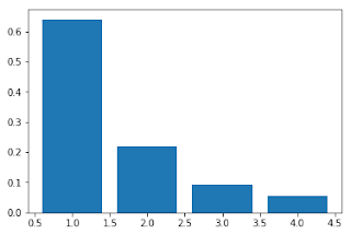


The distribution of flux control is shown below. The vertical axis is the frequency and the x-axis the value of the flux control coefficient from zero to 1.0. The red curve corresponds to the flux control for the first step, on average this has the highest control. The yellow distribution corresponds to the last step of the pathway, you can see it is least likely to have any significant flux control. The conclusion is that given a straight chain with a random set of parameters, on average the first step will have the highest control, progressively decreasing as we work our way down the pathway. Why is this? The explanation is a thermodynamic one which in turn boils down to have easy it is for perturbation to travel up and down the chain. So long as the thermodynamic gradient is from left to right, it is easier for perturbations to propagate downstream compared to upstream. Since flux control is really a measure of how much a perturbation has on the steady-state flux, the easier a perturbation can travel the higher the flux control.

This is not to say that it isn’t possible to get excellent flux control in downstream steps, it’s just that fewer parameter combinations will achieve that.


# Monte Carlo simulation of a straight chain pathway
# Samples parameter values while keeping Keq constant
# Plots the distribution of control coefficients
# Not the most elegant code but I wrote it quickly
 
import tellurium as te
import roadrunner
import random
import pylab as pl
 
r = te.loada("""
   J1: $Xo -> S1; k1*(Xo - S1/Keq1);
       S1 -> S2;  k2*(S1 - S2/Keq2);
       S2 -> S3;  k3*(S2 - S3/Keq3);
       S3 -> $X1; k4*(S3 - X1/Keq4);
     
     k1 = 0.1; k2 = 0.1;
     k3 = 0.1; k4 = 0.1;
     
     Keq1 = 4;
     Keq2 = 3;
     Keq3 = 2;
     Keq4 = 1;
     Xo = 5;
     X1 = 0.1;
""")
 
m = r.simulate (0, 10, 100);
 
aC1 = 0; aC2 = 0; aC3 = 0; aC4 = 0;
aC1a = []; aC2a = []; aC3a = []; aC4a = [];
n = 1000
a = 0
upperLimitK = 50
for i in range (0,n):
    r.setValue ('k1', random.uniform(0, upperLimitK))
    r.setValue ('k2', random.uniform(0, upperLimitK))
    r.setValue ('k3', random.uniform(0, upperLimitK))
    r.setValue ('k4', random.uniform(0, upperLimitK))
    
    try:
      r.simulate()    
      r.steadyState()
      C1 = r.getCC ('J1', 'k1')
      C2 = r.getCC ('J1', 'k2')
      C3 = r.getCC ('J1', 'k3')
      C4 = r.getCC ('J1', 'k4')
      aC1 = aC1 + C1
      aC2 = aC2 + C2
      aC3 = aC3 + C3
      aC4 = aC4 + C4
      aC1a.append (C1)
      aC2a.append (C2)
      aC3a.append (C3)
      aC4a.append (C4)
    except:
        a = a + 1
 
print (aC1/n, aC2/n, aC3/n, aC4/n) 
 
bins = 100
 
pl.hist(aC1a, bins=bins, histtype='stepfilled', density=True, color='r', alpha=0.5, label='C1')
pl.hist(aC2a, bins=bins, histtype='stepfilled', density=True, color='b', alpha=0.5, label='C2')
pl.hist(aC3a, bins=bins, histtype='stepfilled', density=True, color='g', alpha=0.5, label='C3')
pl.hist(aC4a, bins=bins, histtype='stepfilled', density=True, color='y', alpha=0.5, label='C4')
print ("fails = ", a)

Wednesday, December 18, 2019

Stream Plots Using Tellurium

Originally posted on  by hsauro

Every wanted to do a phase plot for a toggle switch or any two-dimensional model? Here is an example of using a stream plot combined with SBML models using Tellurium based on a simple toggle switch.

The colored circles mark the three steady states. The green circle in the middle is on a saddle-node which is unstable (unless you’re exactly on the saddle ridge) and the two on either side are stable nodes.