A simple bistable system

Originally Posted on November 27, 2019 by hsauro

Here is a simple bistable system I sometimes use in class. I like it because it’s easy to explain plus the addition of one extra reaction turns it into a relaxation oscillator.

import tellurium as te
import random
import pylab as plt
import numpy as np

# ---- BISTABLE SYSTEM -----

r = te.loada ('''
     $Xo -> S1;  0.5 + Vmax*S1^n/(15 + S1^n);
      S1 -> ;    k1*S1;

     Xo = 1; S1 = 1;
     n = 4; Vmax = 10; k1 = 2;
''')

plt.xlabel ('Time')
plt.ylabel ('Concentration')
for S1 in np.arange (1.45, 1.55, 0.01):
    r.S1 = S1 
    m = r.simulate (0, 5, 100)
    plt.plot (m['time'], m['[S1]'])
   
r.steadyStateSolver.allow_presimulation = False
for i in range (10):
    r.S1 = random.random()*5
    r.steadyState()
    print ('S1 = ', r.S1, 'eigenvalue = ', r.getFullEigenValues()[0])

If you run the above code you’ll get:

S1 = 5.145227 eigenvalue = -1.84055
S1 = 5.145227 eigenvalue = -1.84055
S1 = 0.251329 eigenvalue = -1.95768
S1 = 5.145227 eigenvalue = -1.84055
S1 = 1.492258 eigenvalue = 3.004970
S1 = 5.145227 eigenvalue = -1.84055
S1 = 1.492258 eigenvalue = 3.004970
S1 = 5.145227 eigenvalue = -1.84055
S1 = 5.145227 eigenvalue = -1.84055
S1 = 0.251329 eigenvalue = -1.957684

The above output is what I call the poor-mans way of finding multiple steady states. I scan across the inital conditions computing the steady state in each case and the corresponding eigenvalue (You can also just assign random values to the initial value for S1, which is better if you don’t know what starting conditions to use). As you can see it found three steady states, two stable (neg eignvalue) and one unstable (1.492, pos eigenvalue).

The plot above shows time course trajectories for about 10 different starting points for S1. The two steady states are clearly evident.

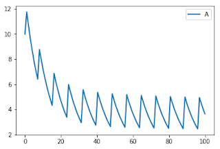
Out of interest here is the addition of the extra reaction at the front to turn it into a relaxation oscillator. You have to make a slight modification to the second reaction’s rate law so that it becomes a function of its reactant (which it wasn’t before)

      $Xo -> So;  k0*Xo;
      So -> S1;   k1*So + Vmax*So*S1^n/(15 + S1^n);
      S1 -> ;     k2*S1;

      Xo = 1; S1 = 1; k0 = 0.07; k1 = 0.04
      n = 4; Vmax = 6; k2 = 0.1;

Simulate Regular Doses using Antimony/SBML in the Tellurium Python Tool

Originally Posted on November 21, 2019 by hsauro

Someone recently asked how to create a model where a molecular species received a regular dose at a fixed interval of 12 hours.

They wanted something where a species A is being degraded but at regular intevals is increased by a fixed amount. See the plot below.

Lucian Smith and I came up with two possible solutions which are shown below. The first solution from Lucian is to set up a variable called trigger that we define using the differential equation trigger’ = 1 (note the apostrophe). The ode ensures that trigger increases linearly during the simulation. We then set up an event that triggers when trigger is greater than 12 hours at which point trigger is set back to zero and we add the dose of value 3 to species A. trigger then starts to integrate again from zero and the cycle repeats.

import tellurium as te

r = te.loada("""
      A ->; k1*A;
      k1 = 0.1; A = 10
      
      trigger = 0
      trigger' = 1

      at (trigger>12): A = A+3, trigger=0
""")

m = r.simulate (0, 100, 100, ['time', 'A'])
r.plot()

The second solution is less elegant but increases the trigger value when an event occurs. In the code below when time exceeds the current trigger value we add the dose then increase trigger by 12 hours so that can it can be triggered again.

m = r.simulate (0, 100, 100, ['time', 'A'])
r.plot()

r = te.loada("""
      A ->; k1*A;
      k1 = 0.1; A = 10
      
      trigger = 12
      at (time > trigger): A = A+3, trigger = trigger + 12
""")

m = r.simulate (0, 100, 100, ['time', 'A'])
r.plot()