Animating pathway

Here is an example of runnign a simulation and plotting the results as an animation. The model is a 20 step linear pathway where at time zero, all concentrations are zero. The boundary species Xo is set to 10 and as the simualtion runs the species slowly fill up to their steady-state levels. We can capture the data and turn it intot an animation using the matplotlib.animation from matlpotlib. At the end we convert the frames into a mp4 file. I generated the model using hte buildnetworks class in teUtils

import tellurium as te
import matplotlib.pyplot as plt
from matplotlib.animation import FuncAnimation, FFMpegFileWriter

r = te.loada('''
J1: $Xo -> S1; e1*(k10*Xo - k11*S1); 
J2: S1 -> S2; e2*(k20*S1 - k21*S2); 
J3: S2 -> S3; e3*(k30*S2 - k31*S3); 
J4: S3 -> S4; e4*(k40*S3 - k41*S4); 
J5: S4 -> S5; e5*(k50*S4 - k51*S5); 
J6: S5 -> S6; e6*(k60*S5 - k61*S6); 
J7: S6 -> S7; e7*(k70*S6 - k71*S7); 
J8: S7 -> S8; e8*(k80*S7 - k81*S8); 
J9: S8 -> S9; e9*(k90*S8 - k91*S9); 
J10: S9 -> S10; e10*(k100*S9 - k101*S10); 
J11: S10 -> S11; e11*(k110*S10 - k111*S11); 
J12: S11 -> S12; e12*(k120*S11 - k121*S12); 
J13: S12 -> S13; e13*(k130*S12 - k131*S13); 
J14: S13 -> S14; e14*(k140*S13 - k141*S14); 
J15: S14 -> S15; e15*(k150*S14 - k151*S15); 
J16: S15 -> S16; e16*(k160*S15 - k161*S16); 
J17: S16 -> S17; e17*(k170*S16 - k171*S17); 
J18: S17 -> S18; e18*(k180*S17 - k181*S18); 
J19: S18 -> S19; e19*(k190*S18 - k191*S19); 
J20: S19 -> $X1; e20*(k200*S19 - k201*X1); 

k10 = 0.86;  k11 = 0.24
e1= 1; k20 = 2.24;  k21 = 0.51
e2= 1; k30 = 2.00;  k31 = 0.49
e3= 1; k40 = 2.54;  k41 = 0.83
e4= 1; k50 = 3.05;  k51 = 0.97
e5= 1; k60 = 1.29;  k61 = 0.10
e6= 1; k70 = 1.94;  k71 = 0.20
e7= 1; k80 = 3.01;  k81 = 0.17
e8= 1; k90 = 0.64;  k91 = 0.19
e9= 1; k100 = 1.96;  k101 = 0.42
e10= 1; k110 = 2.47;  k111 = 0.63
e11= 1; k120 = 4.95;  k121 = 0.51
e12= 1; k130 = 4.78;  k131 = 0.70
e13= 1; k140 = 3.77;  k141 = 0.78
e14= 1; k150 = 1.93;  k151 = 0.37
e15= 1; k160 = 3.87;  k161 = 0.96
e16= 1; k170 = 0.83;  k171 = 0.37
e17= 1; k180 = 1.82;  k181 = 0.69
e18= 1; k190 = 2.62;  k191 = 0.83
e19= 1; k200 = 4.85;  k201 = 0.67
e20= 1; Xo = 10.00
X1 = 0
S1 = 0; S2 = 0; S3 = 0; S4 = 0; 
S5 = 0; S6 = 0; S7 = 0; S8 = 0; 
S9 = 0; S10 = 0; S11 = 0; S12 = 0; 
S13 = 0; S14 = 0; S15 = 0; S16 = 0; 
S17 = 0; S18 = 0; S19 = 0; 
''')

# I'm running this on windows so I had to install the ffmpeg binary
# in order to save the video as an mp4 file
# for more info go tot his page:
# https://suryadayn.medium.com/error-requested-moviewriter-ffmpeg-not-available-easy-fix-9d1890a487d3
plt.rcParams['animation.ffmpeg_path'] ="C:\\ffmpeg\\bin\\ffmpeg.exe"

endTime = 18
fig, ax = plt.subplots(figsize=(8, 5))
ax.set(xlim=(-1, r.getNumIndFloatingSpecies()), ylim=(0, 18))

m = r.simulate(0, endTime, 100)

label = ax.text(15.6, 19, 'Time=', ha='center', va='center', fontsize=18, color="Black")
bars = ax.bar(r.getFloatingSpeciesIds(), m[0,1:], color='b', alpha = 0.5)
    
  def barAnimate(i):
    label.set_text('Time = ' + f'{m[i,0]:.2f}')

    for bar, h in zip(bars, m[i,1:]):
        bar.set_color ('r')
        bar.set_height(h)

anim = FuncAnimation(fig, barAnimate, interval=50, frames=100, repeat=False)

# You can save themp4 file anywhere you want
anim.save('c:\\tmp\\animation.mp4', fps=30)

plt.draw()
plt.show()

This is the resulting video:

Update to teUtils

 I just updated teUtils to version 2.9

UPDATE: The documentation was broken, now fixed. This is a set of utilities that can be used with our simulation environment Tellurium

The update includes some updates to the build synthetic networks functionality. 

The new version adds 'ei*(' terms to mass actions rate laws, eg

S1 -> S2; e1*(k1*S1 - k2*S2)

This makes it easier to compute control coefficients with repect to 'e' I also added a new mass-action rate of the form:

v = k1*A(1 - (B/A)/Keq1)

These can be generated using the call:

model = teUtils.buildNetworks.getLinearChain(10, rateLawType="ModifiedMassAction")

Useful if you want to more easily control the equilbrium constant for a reaction. Here is an example of a three step random linear chain:

model = teUtils.buildNetworks.getLinearChain(10, rateLawType="ModifiedMassAction")
print (model)

J1: $Xo -> S1; k1*Xo*(1 - (S1/Xo)/Keq1); 
J2: S1 -> S2; k2*S1*(1 - (S2/S1)/Keq2); 
J3: S2 -> $X1; k3*S2*(1 - (X1/S2)/Keq3); 

k1 = 1.42;  Keq1 = 3.61
e1 = 1; k2 = 1.42;  Keq2 = 7.91
e2 = 1; k3 = 3.50;  Keq3 = 5.64
e3 = 1; Xo = 5.00
X1 = 0
S1 = 1E-6; S2 = 1E-6; 

Executing tellurium models in a sphinx document

I needed to be able to generate simulation plots for a sphinx document but I didn't want to have to generate the plots separately and then include them manually.  I wanted the simulations done from within sphinx so that they would be automatically included when building the document. The key to this is to add the following to the list of extensions in the sphinx conf.py file:

extensions.append ('matplotlib.sphinxext.plot_directive')

To use it in a sphinx document use the plot directive, for example:

.. plot::
   :include-source:

   import tellurium as te
   r = te.loada ('''A -> B; k1*A; k1=0.1; A = 10''')
   m = r.simulate (0, 40, 100)
   r.plot()

It assumes you have matplotlib installed in your python setup (I am using Windows 10, Python 3.11). Further  information can be found here:

https://matplotlib.org/stable/api/sphinxext_plot_directive_api.html

How to execute python code in a sphinx document

This is a note for myself but others might find useful.  I needed to execute python in a sphinx document at build time. 

The package that comes up in a search doesn't work with Python 3.x. 

Instead I found 

https://pypi.org/project/sphinx-execute-code-python3/ 

which does work with Python 3.11. (I'm running Windows 10)

Install it by typing the following on the command line

pip install sphinx-execute-code-python3 

To use it don't forget to add this line to your sphinx conf.py file:

extensions.append('sphinx_execute_code')

Here is an example in a rst file:

.. execute_code::

    a = [1,2,3]

    b = [4,5,6]

    print ('Printing a list: ', a + b)

The docs have various options you can use.

A simple linear pathway

Analysis of a simple pathway:

This model is model a) from the paper by Tyson et al (2003) "Sniffers, buzzers, toggles and blinkers: dynamics of regulatory and signaling pathways in the cell". I changed their R to P however so I could use the symbol R for response.

Assume $ v_1 = k_1 S $ and $ v_2 = k_2 P $ Then $\frac{dP}{dt} = k_1 S - k_2 P $. At steady-state this equals 0 so that $$ P = \frac{k_1 S}{k_2} $$ In other words P is a linear function of S. In terms of logarithmic senstivities or the reponse coefficient: $$ R^P_S = \frac{dP}{dS} \frac{S}{P} = \frac{k_1}{k_2} \frac{k_2}{k_1} = 1 $$ That is a 1% change in S will lead to a 1% change in the steady-state level of P. This is important because in their pathway (d, shown below) they use this property to ensure that when S also regulates a secondary pathway that in turn up regulates the consumption step v2, the level of P remains unchanged.

This property is not very robust however and any change to the rate law on $v_1$ will result in the pathway failing to maintain P constant. For example if $v_1 = k_o + k_1 S$, where we've added a basal rate of $k_o$, then the response becomes: $$ R^P_S = = \frac{k_1 S}{k_o + k_1 S} $$ that is the response is no longer proportional. Change S in this case will result in P changing. The code below will model this system. One important point to make is that this isn't an example of integral control.

import tellurium as te
import matplotlib.pyplot as plt
  
r1 = te.loada("""
     -> P; k0 + k1*S
     P ->; k2*X*P
     -> X; k3*S
     X ->; k4*X
     
     k1 = 1; k2 = 1
     k3 = 1; k4 = 1
     
     # Set basal rate to zero 
     k0 = 0; S = 1
     
     # Change signal, P won't change
     at time > 10: S = S*2
     
     # Change basal rate and set S back to what it was
     at time > 25: k0 = 0.3, S = 1;
     
     # Change signal, this time P will change
     at time > 40: S = S*2      
""")

m = r1.simulate(0, 60, 200, ['time', 'P', 'S'])
plt.plot (m['time'], m['P'], label='P')
plt.plot (m['time'], m['S'], label='S')
plt.text(2, 0.75, "Basal = 0")
plt.text(9, 0.9, "Change S")
plt.text(14, 1.2, "P restored")
plt.text(20, 0.75, "Set basal > 0")
plt.text(35, 0.9, "Change S, P not restored")
plt.legend()

Plotting a steady-state plot

It's always surprising to find students who don't quite get what a steady-state is. Here is a simulation of a three step pathway that might help. You'll need to install tellurium for this to work.

$X_o \stackrel{v_1}{\rightarrow} S_1 \stackrel{v_2}{\rightarrow} S_2 \stackrel{v_3}{\rightarrow}$

we assume that $X_o$ is fixed and does not change in time. I don't care where $S_3$ goes.

If we start with zero concentrations for $S_1$ and $S_2$ we get the following plots. The left plot shows the change in concentration and the right plot the reaction rates. Note that all three reaction rates approach the same rate since at steady-state all rates must be equal.

Here is the python code that will generate that plot. To get the reaction rate symbols above the reaction arrows I used a bit of a hack by printing two text strings, one above the other. For some reason I couldn't get matplotlib to recognise the LaTeX command stackrel.

import tellurium as te
import matplotlib.pyplot as plt

r = te.loada("""
    J1: $Xo -> S1; k1*Xo - k2*S1
    J2:  S1 -> S2; k3*S1 - k4*S2
    J3:  S2 -> ;   k5*S2
      
      k1 = 0.1; k2 = 0.04
      k3 = 0.14; k4 = 0.09
      k5 = 0.16
      Xo = 10
""")

m = r.simulate (0, 60, 100)
plt.subplot (1,2, 1)
plt.plot(m['time'], m['[S1]'], label='S1')
plt.plot(m['time'], m['[S2]'], label='S2')
plt.ylim((0, 9))
plt.xlabel('Time')
plt.ylabel('Concentration')
plt.text(5, 8.4, 'Approach to steady-state')
plt.text(5, 7.8, '$X_o$ is fixed')
plt.text(14, 1.5, r'$\quad\  v_1 \quad v_2 \quad v_3$', fontsize = 12) 
plt.text(14, 1, r'$X_o \rightarrow S_1 \rightarrow S_2 \rightarrow$', fontsize = 12) 
plt.legend(bbox_to_anchor=(0.4, 0.5))

# Next generate the reaction rates
r.reset()
m = r.simulate (0, 40, 100, ['time', 'J1', 'J2', 'J3'])
plt.subplot (1,2, 2)
plt.plot(m['time'], m['J1'], label='$v_1$')
plt.plot(m['time'], m['J2'], label='$v_2$')
plt.plot(m['time'], m['J3'], label='$v_3$')
plt.xlabel('Time')
plt.ylabel('Flux')
plt.text(14, 0.2, r'Reaction rates', fontsize = 12) 
plt.legend()
plt.tight_layout()
plt.show()

1888 Math Exam

Nothing to do with cells or modeling, but I recently purchased a 1885 copy of John Casey's rendition of Euclid's Elements. John Casey was born in Limerick, Ireland, and became a lecturer in mathematics at University College Dublin. He wrote one of the more well-known editions of Euclid's elements. In his preface he states:

"This edition of the Elements of Euclid, undertaken at the request of the principals of some of the leading Colleges and Schools of Ireland, is intended to supply a want much felt by teachers at the present day—the production of a work which, while giving the unrivalled [sic] original in all its integrity, would also contain the modern conceptions and developments of the portion of Geometry over which the Elements extend."

You can find a copy at Project Gutenberg (https://www.gutenberg.org/ebooks/21076) if you are curious. 

What's interesting about the book I received, is not so much the geometry, but what I found inside. 

Inside was a copy of a math Pass Examination paper from 1888, presumably from University College Dublin but at least somewhere in Ireland (I purchased the book from Dublin). Update: There are two inscriptions in the book. The first is a simple "W.H Dunlop May 1886".  The second is more interesting and written in a very elegant cursive style where the book was transferred two years later to: Michael J Buckley. Catholic University Dublin. 19.1.'88. This is the name of the first university dedicated to accepting Catholics from Ireland (Trinity College was the Anglican University founded by Elizabeth I, so you can imagine the problem). However, the university didn't do too well financially and had problems awarding degrees because it didn't have a royal charter. In 1908/1909, it became the University College Dublin with its own charter. 

The exam had 10 questions, one involving reaping a field, another about selling a horse, and another about carpeting a room. The remaining 7 are pure math questions, with a number of them being numerical estimation questions, eg, roots, squares etc. I think modern students could do these questions, though they might struggle with the numeric computations unless they have a calculator at hand. I took a photograph of the exam for all to see:

Optimal distribution of enzymes that maximizes flux

Here is an interesting metabolic question to ask. Consider a pathway with two steps: $$\large X_0 \stackrel{e_1}{\rightarrow} S \stackrel{e_2}{\rightarrow} $$ where the first step is catalyzed by enzyme $e_1$ and the second step by $e_2$. We can assume that a bacterial cell has a finite volume, meaning there is only so much space to fit all the proteins necessary for the bacterium to live. If the cell make more of one protein, it presumably needs to find the extra space by down expressing other proteins. If the two step pathway is our cell, this translates to there being a fixed amount of protein that can be distributed betwen the two, that is: $$ e_1 + e_2 = e_t $$ Presumably evolutionary pressure will maximize the flux through the pathway per unit protein. This means that given a fixed total amount of protein $e_t$ there must be a particular distribution of protein between $e_1$ and $e_2$ that maximizes flux. For example, if most of the protein were allocated to $e_1$ and very little to $e_2$ then the flux would be quite low. Likewise if most of the protein were allocated to $e_2$ and very little to $e_1$ then again the flux would be low. Between these two extremes there must be a maximum flux. To show this is the case we can do a simple simulation shown in the python code below. This code varies the levels of $e_1$ and $e_2$ in a loop such that their total is always 1 unit. Each time we change $e_1$ we must change $e_2$ by the same amount in the opposite direction in order to keep the constant fixed. As we do this we collect the steady-state flux and the current level of $e_1$. Finally we plot the flux versus $e_1$.

import tellurium as te
import roadrunner
import matplotlib.pyplot as plt

r = te.loada("""
     J1: $Xo -> S; e1*(k1*Xo - k2*S)
     J2: S ->; e2*k3*S
     
     Xo = 1
     k1 = 0.5; k2 = 0.2
     k3 = 0.45
     e1 = 0.01; e2 = 0.99
""")

r.steadyState()

x = []; y = []; 
for i in range (49):
    r.e1 = r.e1 + 0.02
    r.e2 = 1 - r.e1  # Total assumed to be one
    r.simulate()
    r.steadyState()
    x.append (r.e1)
    y.append (r.J1)
    
plt.figure(figsize=(12,10))
plt.grid(b=True, which='major', color='#666666', linestyle='-')
plt.grid(b=True, which='minor', color='#999999', linestyle='-', alpha=0.2)
plt.minorticks_on()
plt.plot (x, y, linewidth = 2)
plt.xlabel('$e_1$', fontsize=36)
plt.ylabel('Flux', fontsize=36)

 

The following graph show the results from the simulation (the font sizes might be on the big size if you have a low res monitor):

You can see the flux reaching a maximum at around $e_1 = 0.6$, meaning also that $e_2 = 0.4$ in order to keep the total fixed. The actual position of the peak wil depend on the rate constants in the rate expressions. Let's assume we are at the maxium. The slope, $dJ/de_1$, at the maxium is obviously zero. That means if we were to move a small amount of protein from $e_1$ to $e_2$ the flux won't change. We can write this experiment in terms of the two flux control coefficients: $$ \frac{\delta J}{J} = 0 = C^J_{e_1} \frac{\delta e_1}{e_1} + C^J_{e_2} \frac{\delta e_2}{e_2} $$ However, we know that in this particlar experiment the change in $e_1$ is the same but oppisite to the change in $e_2$. That is $\delta e_1 + \delta e_2 = 0$ or $$ \delta e_1 = -\delta e_2$$ Replacing $e_2$ with $-\delta e_1$ gives: $$ \frac{\delta J}{J} = 0 = C^J_{e_1} \frac{\delta e_1}{e_1} - C^J_{e_2} \frac{\delta e_1}{e_2} $$ $$ \frac{\delta J}{J} = 0 = C^J_{e_1} \frac{1}{e_1} - C^J_{e_2} \frac{1}{e_2} $$ $$ C^J_{e_1} \frac{1}{e_1} = C^J_{e_2} \frac{1}{e_2} $$ Giving the final result: $$ \frac{C^J_{e_1}}{C^J_{e_2}} = \frac{e_1}{e_2} $$ That is, when the protein distribution is optimized to maximize the flux, the flux control coefficients are in the same ratio as the ratio of enzyme amounts. This generalizes to any size pathway with multiple enzymes. This gives us a tantgilizing suggestion that we can obtain the flux control coeficients just by measuring the protein levels.

There is obviously a lot more one can write there and maybe I do that in future blogs but for now you can get further information:

S. Waley, “A note on the kinetics of multi-enzyme systems,” Biochemical Journal, vol. 91, no. 3, p. 514, 1964.

J Burns: “Studies on complex enzyme system.” https://era.ed.ac.uk/handle/1842/13276, 1971 (page 141-) I have a LaTeX version at: https://github.com/hsauro/JumBurnsThesis

Guy Brown, Total cell protein concentration as an evolutionary constraint on the metabolic control distribution in cells,” Journal of theoretical biology, vol. 153, no. 2, pp. 195–203, 1991.

E. Klipp and R. Heinrich, “Competition for enzymes in metabolic pathways:: Implications for optimal distributions of enzyme concentrations and for the distribution of flux control,” Biosystems, vol. 54, no. 1-2, pp. 1–14, 1999

Sauro HM Systems Biology: An Introduction to Metabolic Control Analysis, 2018

Relationship of fluxes to enzyme levels in a metabolic pathway

To get hold of me it is best to contact me via my email address at: hsauro@uw.edu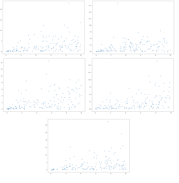

Someone asked me the other day what the relationship was between the steady-state fluxe through a reaction and the coresponding level of enzyme. Someone else suggested that there would be a linear, or proportional relatinship between a flux and the enzyme level. However, this can’t be true, at least at steady. Considder a 10 step linear pathway. At steady-state each step in the pathway will, by defintion, carry the same flux. This is true even if each step has a different enzyme level. Hence the relationship is so simple. In fact the flux a given step carries is a systemic properties, dependent on all steps in the pathway. As an experiment I decided to do a simulation on some synthetic netowrks with random parameters and enzyme levels. For this exmaple I just used a simple rate law of the form: $$ v = e_i (k_1 A - k_2 B) $$ For a bibi reaction, A + B -> C + D, the coresponding rate law would be: $$ v = e_i (k_1 A B - k_2 C D) $$ a similar picture would be seen for the unibi and biuni reactions. Using our teUtils package I generated random networks with 60 species and 150 reactions. The reactions allowed are uiui-uinbi, biui or bibi. I then randomized the values for the enzymne levels $e_i$ and computed the steady-state flux. I used the following code to do the analysis. I have a small loop that generates 5 random models but obviously this number can be changed. I generate a random model, load the model into roadrunner, randomize the values for the $e_i$ parameters between 0 and 10, compute the steady-state (I do a presimulation to help things along) and collect the corresponding $e_i$ and flux values. Finally I plot each pair in a scatter plot.

import tellurium as te
import roadrunner
import teUtils as tu
import matplotlib.pyplot as plt
import random


for i in range (5):
    try:
      J = []; E = []
      antStr = tu.buildNetworks.getRandomNetwork(60, 150, isReversible=True)
      r = te.loada(antStr)

      n = r.getNumReactions()
      for i in range (n):      
          r.setValue ('E' + str (i), random.random()*10)    
      m = r.simulate(0, 200, 300)
      r.steadyState()

      for i in range (n):
          J.append (abs (r.getValue ('J' + str (i)))) 
          E.append (r.getValue ('E' + str (i)))        
      
      plt.figure(figsize=(12, 8))
      plt.plot(E, J, '.')
        
    except:
        print ('Error: bad model')

The results for five random networks is shown below. Note the x axis is the enzyme level and the y axis the corresponding steady-state flux through that enzyme. It's intersting to see that there is a rough correlation between enzyme amount and the corresponding flux, but its not very strong. Many of the points are just scattered randomly with some showing a definite correlation. The short answer is the realtinship is not so simple.

How not to Comment Code

I recently came across one of the ten simple rules aricles in PLoS Comp Bio:

"Ten simple rules for tackling your first mathematical models: A guide for graduate students by graduate students" by Korryn Bodner et al

https://journals.plos.org/ploscompbiol/article?id=10.1371/journal.pcbi.1008539

One thing that struck me was Rule 5 on coding best practices with commenting being one of the discussion points. What struck me was their screen shot of a documented function shown below (in R):

My take on commenting is that it should be used to add human readable metadata on elements of a program that are not immediately obvious.

Most of the time, code should be sufficiently readable to indicate what it's doing. Obviously some languages are better than others when desribing an algorithm but it is also dependent on the programmer. I've seen code written in clear languages that are unintelliglbe, but I've also seen code written in poorly expressible languages that are easily readable. Although the programming language itself can influence code reability I think the programmer has much more influence.

But back to Rule 5. In the example you'll see something like:

# calculate the mean of the data

u <- mean (x)

This is completely redundant, as the coding states what it is going to do. In fact the authors comment every line like this. If anythng, I think the extent of comments actually hinders the reabilty of the code. The code itself is mostly clear as to what it is doing. There may be a justification to include a comment on next line that computes the standard error because the variables names are so badly chosen, e.g what does the following line do:

s <- sd(x)

sd might stand for standard deviation but the rest of the line offers no clue. If it had been written as:

standardDeviation <- sd(x)

It would have been much clearer, instead the authors add a comment to make up for poor choice of variable names. They also give the function itself a nondescriptive name, in this case ci. It would have been better to write the function using getConfidenceInterval or similar:

getConfidenceInterval <- f (data) {

etc

Euclid's Elements

Nothing to do with cells and networks, but I have an interest in Euclid's Elements and decided to publish a new edition of Book I. The difference with previous editions is that this one is in color and also has a chapter on the history of the elements, together with commentaries on each proposition. For those unfamiliar with Euclid's Elements, it's a series of books (more like chapters in today's language) laying the foundation for geometry and number theory. Book I focuses on the foundation of geometry culminating in a proof for Pythagoras' theorem and other important but less known results. The key innovation is that it describes a deductive approach to geometry. It starts with definitions and axioms from which all results are derived using logical proofs.

It occurred to me that something similar could be done with deriving the properties of biochemical networks. For example, we might define the following three primitives:

I. Species

II. Reaction

III. Steady-state

We might then define the following axioms:

I. A species has associated with it a value called the concentration, x_i.

II. All concentrations are positive.

III. A reaction has a value associated with it called the reaction rate, v_i.

IV. Reaction rates can be negative, zero, or positive.

V. A reaction transforms one or more species (reactants) into one or more other species (products).

VI. The reaction rate is a continuous function of the reactants and products.

VII. The rate of change of a species can be described using a differential equation, dx/dt

VIII. All steps are reversible unless otherwise stated (may this can be derived?)

etc

Given these axioms, we could build a series of propositions. This might be an interesting exercise to do. Some of the more obvious propositions would be the results from metabolic control analysis, such as the summation and connectivity theorems.

Link to Amazon