Plotting a steady-state plot

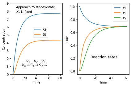
It's always surprising to find students who don't quite get what a steady-state is. Here is a simulation of a three step pathway that might help. You'll need to install tellurium for this to work.

$X_o \stackrel{v_1}{\rightarrow} S_1 \stackrel{v_2}{\rightarrow} S_2 \stackrel{v_3}{\rightarrow}$

we assume that $X_o$ is fixed and does not change in time. I don't care where $S_3$ goes.

If we start with zero concentrations for $S_1$ and $S_2$ we get the following plots. The left plot shows the change in concentration and the right plot the reaction rates. Note that all three reaction rates approach the same rate since at steady-state all rates must be equal.

Here is the python code that will generate that plot. To get the reaction rate symbols above the reaction arrows I used a bit of a hack by printing two text strings, one above the other. For some reason I couldn't get matplotlib to recognise the LaTeX command stackrel.

import tellurium as te
import matplotlib.pyplot as plt

r = te.loada("""
    J1: $Xo -> S1; k1*Xo - k2*S1
    J2:  S1 -> S2; k3*S1 - k4*S2
    J3:  S2 -> ;   k5*S2
      
      k1 = 0.1; k2 = 0.04
      k3 = 0.14; k4 = 0.09
      k5 = 0.16
      Xo = 10
""")

m = r.simulate (0, 60, 100)
plt.subplot (1,2, 1)
plt.plot(m['time'], m['[S1]'], label='S1')
plt.plot(m['time'], m['[S2]'], label='S2')
plt.ylim((0, 9))
plt.xlabel('Time')
plt.ylabel('Concentration')
plt.text(5, 8.4, 'Approach to steady-state')
plt.text(5, 7.8, '$X_o$ is fixed')
plt.text(14, 1.5, r'$\quad\  v_1 \quad v_2 \quad v_3$', fontsize = 12) 
plt.text(14, 1, r'$X_o \rightarrow S_1 \rightarrow S_2 \rightarrow$', fontsize = 12) 
plt.legend(bbox_to_anchor=(0.4, 0.5))

# Next generate the reaction rates
r.reset()
m = r.simulate (0, 40, 100, ['time', 'J1', 'J2', 'J3'])
plt.subplot (1,2, 2)
plt.plot(m['time'], m['J1'], label='$v_1$')
plt.plot(m['time'], m['J2'], label='$v_2$')
plt.plot(m['time'], m['J3'], label='$v_3$')
plt.xlabel('Time')
plt.ylabel('Flux')
plt.text(14, 0.2, r'Reaction rates', fontsize = 12) 
plt.legend()
plt.tight_layout()
plt.show()