Converting Excel Tables to LaTeX Tables

Originally Posted on December 29, 2013 by hsauro

Today I had the problem of converting an Excel table of values into a LaTeX table. I could have done it by hand but the table had over 400 entries so that would have been a bit tedious. Instead I did the usual and hunted around for any automated possibilities and came across two:

1. Excel2LaTeX.

This is a Excel Add-In that converts a selected set of Excel rows and columns into a LaTeX table. However as per usual for Microsoft it isn’t trivial to add Add-Ins. After some fuzzing around I discovered these instructions on stackoverflow. One would think that adding an Add-In to Excel would be a case of simply loading the Add-In file, but of course not, it requires a minimum of at least 8 different steps. But it doesn’t end there. The final step, number 9, is to close Excel, yes I said close Excel, restart Excel and the Add-In is available (hopefully). After that the Add-In is fairly trivial to use and offers a number of useful formating options..

2. The second option is an online tool by Eric Wood This was very easy to use, just drag your excel file on the the browser window. If your data is on a particular sheet, make sure to select that sheet on the provided dropdown list.

Converting Excel Tables to LaTeX Tables

December 29, 2013 6:31 pm

Today I had the problem of converting an Excel table of values into a LaTeX table. I could have done it by hand but the table had over 400 entries so that would have been a bit tedious. Instead, I did the usual and hunted around for any automated possibilities and came across two:

1. Excel2LaTeX.

This is a Excel Add-In that converts a selected set of Excel rows and columns into a LaTeX table. However as per usual for Microsoft it isn't trivial to add Add-Ins. After some fuzzing around I discovered these instructions on stackoverflow. One would think that adding an Add-In to Excel would be a case of simply loading the Add-In file, but of course not, it requires a minimum of at least 8 different steps. But it doesn't end there. The final step, number 9, is to close Excel, yes I said close Excel, restart Excel and the Add-In is available (hopefully). After that, the Add-In is fairly trivial to use and offers a number of useful formatting options..

2. A second option is an online tool by Eric Wood This was very easy to use, just drag your excel file on the browser window. If your data is on a particular sheet, make sure to select that sheet on the provided dropdown list.

Bottlenecks and Slow Steps - again

October 28, 2013 5:55 pm

I've written a few articles on this blog about the irrationality of bottlenecks and slow steps in metabolism, hoping that one day my fellow scientists will feel the same. Sadly it is not true and maybe I should write more because I week or two ago I came from a talk about metabolic engineering which made some egregious statements that I wouldn't even expect my undergraduates to make. Apparently *the* bottleneck (note singular) in a metabolic pathway is the 'slowest' step and that's the one to engineer. I should add that this not quite right. Unfortunately I've no idea what they meant by the slowest step and I didn't have the heart to ask them given how lost they were. If I did ask, I suspect they'd become even more confused.

I think its time to write a blog on "What's the deal with slow steps"'

How to Increase MikTeX 2.9 Memory

Originally Posted on August 12, 2013 by hsauro

I was recently running some large stochastic simulations and was generating very large pgfplot data files. MikTeX out of the box was unable to compile these plots because it kept running out of main memory. To increase main memory (or other memory limits) run the following line from the DOS prompt:

initexmf --edit-config-file pdflatex

This will open the configuration file for pdflatex into an editor (probably notepad). Add the following lines to this configuration file:

pool_size=5000000
main_memory=6000000
extra_mem_bot=2000000
font_mem_size=2000000


I needed lots of memory so these numbers are quite bit. I’ve got 8GB of RAM so let’s be generous (My first computer was the MK14 which had 256 bytes of RAM, things have moved on a little).

Save the file (file name is provided) and then remake the format files. To do this use the command line:

initexmf --dump=pdflatex

I happen to use pdflatex all the time so note that I am specifying pdflatex in each of the commands. If you’re using straight latex then substitute pdflatex with latex.

Talking about big tikz/pfdplot figures, don’t forget to use the external command:

\usepackage{tikz}
\usetikzlibrary{external}
\tikzexternalize % activate!


This forces tikz to reuse previously stored figures, saves regenerating them all the time. See section 32 of the TikZ manual (Version 2.10 !) for more details.

Filming Paramecium bursaria

July 13, 2013 5:16 pm

I got myself a camera attachment from AmScope for the relatively cheap microscope I have (A OMAX 40X-2000X Digital Binocular Biological Compound Microscope - find it on Amazon). I used my wife's Cannon 3Ti to take the video. Got some water form one of my plant trays and had a look. Not much life, a few unidentified and quite small ciliates, a few Euglena, some unidentified filamentous algae and what looked like some spirochetes. But what caught my attention was one Paramecium and not any old Paramecium but a Paramecium called Paramecium bursaria. What is interesting about this particular Paramecium is that it has a symbiotic relationship with green algae called Zoochlorella.

The video below (taken at roughly 600x to 800x) shows a number of interesting features, some of which I've never seen myself before and it was very interesting when I realized what was going on. In the video you'll see two contractile vacuoles pumping water out of the cell, a large nucleus near the center and an oral grove to the left of the nucleus with some beating cilia. Also notice the many symbiotic algae in the cell. Also around the outside of the Paramecium you'll also see beating cilia. The entire cell is about 100 to 150 microns long. It took a while for the cell to settle down so that I could photograph it. One question, in the first image you'll see some long thin algae (?) like cells drifting from the top to the bottom left corner. I have not been able to identify these but the sample was full of them and I suspect is what gave the water a slightly green color.

Linear Dynamics Application

May 16, 2013 9:22 am

There are a number of online apps that can show students the phase plane dynamics of a 2d system. Notable examples include:

Phase Portrait Viewer from the d’Arbeloff Interactive Math Project - requires Java installed
Wolfram Phase Portrait Viewer - required Mathematica CDF Installed
Programmable Interactive Simulator (DField and PPlane) - requires Java (Matlab version also available I believe)

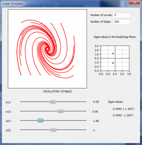
Nevertheless, I decided, just for the hell of it to write my own, this time a desktop application for windows. Screenshot and download link below:

The download is below. Nothing to install, the application is a single exe that you just run. Works on Windows and Wine emulator.

Download linear dynamics simulator

Written using Delphi XE.

Drawing Pathways with Tikz

Originally Posted on May 8, 2013 by hsauro

I had the need to draw a negative feedback around a linear pathway. Normally I would use a vector drawing packages to do this, such as Illustrator or Inkscape. This time I thought I would try the tikz package that allows one to embed diagrams inside LaTeX files in script form. The tikz manual is an excellent source of ideas and in one section they show how to draw syntax diagrams (Section 5, page 60). I re-purposed some of this code to draw the following pathway with a negative feedback:

To draw this diagram I used the following code. The code is split into fours sections. The header and three coding sections. The first coding section places and names the four species nodes. Naming nodes is very used later on. The second section draws the reaction arrows and the final section draws the negative feedback loop. The header specifies the type of arrow that will be used, >=latex’ which is the latex arrow (See section 23, page 256 for more choices of arrows), and the distance between nodes. See the comments in the code to understand how the feedback loop was made.

\begin{tikzpicture}[>=latex', node distance=2cm]

\node (Xo) {\Large $X_o$};
\node [right of = Xo] (S1) {\Large $S_1$};
\node [right of = S1] (S2) {\Large $S_2$};
\node [right of = S2] (X1) {\Large $X_1$};

\draw [->,ultra thick,blue] (Xo) -- node[above, black] {$v_1$} (S1);
\draw [->,ultra thick,blue] (S1) -- node[above, black] {$v_2$} (S2);
\draw [->,ultra thick,blue] (S2) -- node[above, black] {$v_3$} (X1);

% Lets draw a line with a blunt end, -|
\draw [-|,ultra thick,blue]
% start in the middle of S2, and move down 2.75 mm 
% ($ ... $) notation is used to add the coordinates
($ (S2) + (0mm,-2.75mm) $)
% Now draw the line down by 3mm
% -- means draw to, + means move by 
-- +(0,-3mm)
% Now move back to the left of S2
% The symbol -| means draw horizontal then vertical. 
% If we used -- instead the line would be drawn 
% diagonally to the reaction edge.
% (S1) is the center of the node. But we want the
% blunt end to end below the S1 line and
% half way to the left. The 10mm is half the node
% distance of 2cm, and 1mm is slightly below  
% the reaction line.
-| ($ (S1) - (10mm,1mm) $);

\end{tikzpicture}

-1 times -1 = +1 ?

Originally Posted on April 21, 2013 by hsauro

Lost Blog

My brother asked me the other day why -1 times -1 was +1. It’s the sort of rule we learn at high school and perhaps never think about again. I thought I’d add a note to prove and show why....

The easiest way to think about this is that a negative will negate the other term. This, -1 times +1 will negate the +1 giving -1. We can use the same argument to suggest that -1 times -1 means that the first -1 negates the second -1 leading to +1.

More formally we call also use the following proof:

Consider:

$$ (-1) \times (-1 + 1) $$

We can look at this in two ways:

1) Use the distributive law to expand the expression:

$$ (-1 \times -1) + (-1 \times 1) $$

2) Evaluate the term $(-1 + 1)$:

$$ (-1) \times (0) = 0 $$

Therefore the expression $(-1) \times (-1 + 1) $ equals zero, that is:

$$ (-1 \times -1) + (-1 \times 1) = 0 $$

If we agree that $(-1 \times 1) = -1$ then
$$ (-1 \times -1) = 1 $$

Note that if we were to assert that in fact $-1 \times -1 = -1$, then assuming the distributive law is valid we end up with an inconsistent answer:

$$ (-1) \times (1 + -1) = (-1) \times (1) + (-1) \times (-1)$$

Assuming now that $-1 \times -1 = -1$, we then obtain:

$$ (-1) \times 0 = -1 + -1 = 2$$

That is:

$$ 0 = -2 $$

We would only get a sensible answer if we also assumed that $-1 \times 1 = 1$ which doesn't seem reasonable at all.

See the MathForum for examples.

Choke points, Load points, Hots spots and Key steps

March 23, 2013 8:56 pm

Choke points, load points, hot spots, key steps and critical steps are some of the many phrases that have been coined to describe places in a biochemical network where perturbations are said to make a difference. Locating these places is important because they are sites where we would target a drug or reengineer to change a cell's phenotype. The question is what are these points, is a choke point something that can be identified as a physical thing, can a choke point be removed from a pathway and studied in isolation? To answer these questions let us look at a very simple two step pathway. Both steps in the pathway are governed by reversible Michaelis-Menten kinetics, so nothing out of the ordinary. Let's say that a perturbation to the enzyme activity at the second step results in a significant change in the steady-state flux through our little pathway, The first step has hardly any effect. We might therefore call the second step the choke point of the pathway, or the rate-limiting step, the hot spot etc.

Is there something special about the second step that makes it a 'choke point'? What may surprise many is that it is the first step that makes the second step a choke point. There is nothing intrinsically special about the second step that makes it the choke point, all the interesting action occurs at the first step.

The explanation is simple. The reaction rate through the first step is very sensitive to the product it makes. If the product of the first step goes up a bit the result is that the reaction rate through the first step goes down, this is simply due to strong product inhibition, that is the product is an effective competitor with respect to the substrate for the first step. So what? Consider this scenario, we add a drug that can inhibit the activity of the second step. Its reaction rate goes down. This results in the substrate for the second step to go up (its being consumed less so it must go up). Since the first step is sensitive to this concentration, its rate goes down. The net effect is that it looks as if the second step is the choke point. The name choke suggests a small diameter pipe so that making the pipe smaller has a marked effect on the flow. But this isn't what is happening here. What is happening is that there is negative feedback from the second step to the first step and it is the first step that slows down the flow. If it weren't for the product inhibition on the second step, the second step would have NO effect on the flow. The second step is actually NOT a choke point at all.

The words we use can be very misleading especially when dealing with complex systems. In this case the work choke is extremely misleading. What about the other phrases that people use, such as a hot spot. Hot spot is certainly a colorful phrase to use but is it a phrase that should be used by intelligent people? Its certainly a word that politicians or my 4 your old might understand, but is it a word that professional scientists should use? What about the word key step or critical step? These don't convey the point that the step itself is not the one responsible for it being influential, it was the first step that gave the second step its ability to control flux. If anything the key step is the first step. These words aren't therefore really appropriate either. What about the word rate-limiting step, still in use today in some circles? That word also suggests a pipe that is too small to carry the flow, it has the same problem as the word choke point.

Most of the words we use are either imprecise or just misleading. What do we use instead? As scientists we should define precisely what we mean, preferably operationally and quantitatively. Forty years ago such a definition was given, that definition is the flux control coefficient, it is simply a number that tells us how much of an effect a perturbation has on the system as a whole. It doesn't explain why a particular step has a given a degree of influence, it just tells us how much influence the step has.

Metabolic pathways such as the amino acid biosynthetic pathways which have allosteric negative feedback are an interesting case. The old literature (and even some new literature) will refer to the step that is regulated by the allosteric effector the rate-limiting step, the choke point or hot spot in more recent language. But modifying this step actually has little effect on the phenotype. It turns out that its the step after the feedback loop that has most of the influence. However it is the regulated step that allows influence to be on the last step. The allosterically regulated step is an important step but it certainly isn't the rate-limiting step, choke point or hot spot.

A real choke point, The Battle of Thermopylae.
Leonidas at Thermopylae, by Jacques-Louis David, 1814.
Image and data provided by Columbia University.

 

Irreversible Bistability

March 17, 2013 8:40 pm

Last week I was in need of an irreversible bistable switch to show my class. I remember seeing one in the well-known review by Tyson et al, Sniffers, buzzers, toggles and blinkers: dynamics of regulatory and signaling pathways in the cells, Current Opinion in Cell Biology 2003, 15:221–231. I hunted down the paper and found it. However, when I looked at the details of the model, it turns out to be incorrect or at least very odd. I couldn't get the model to work and I didn't particularly like the equations that described the model (assuming they were correct and not a typo in the paper). So I decided to design my own. The traditional bistable system has two physically realizable steady states, that is states that admit positive concentrations. By suitably large perturbations it is possible to jump from one state to the other. We often depict bistable systems in the form of a bifurcation diagram as shown below:

Here we see the state of the system (vertical axis) plotted as a function of a parameter in the system. Over a particular range of the parameter, we see that the system admits three possible solutions (along a vertical line). Two are stable and the third is unstable (blue dotted line). If I start on at a high steady-state at a parameter value of say 1.2 and slowly increase the parameter, the steady-state value will slowly decrease until I reach a parameter value of about 2.4 where we suddenly jump to the lower steady state. If I now decrease the parameter value I now follow the lower steady-state branch until I reach about 1.3 where I will suddenly jump up to the high state. I can therefore move freely between the high state and the low state simply by changing the parameter. The bistable system is therefore freely reversible.It is possible however to arrange things so that the entire curve is shifted to the left in such a way that is becomes impossible to freely move back and forth between the states.

In the above diagram, we see that the left-hand turning point now pokes into the negative half of the graph. The graph is mirror image of the previous one because I used a slightly different model in the upper one, but don't let that worry you. The negative half implies negative concentrations which is clearly impossible. Consider then starting the parameter (this time called the signal) at zero with the variable also at zero and slowly increasing the signal level. The output concentration will slowly increase following the lower branch until we reach a signal value of about 2.0 when we suddenly jump to the high state. Let us now start lowering the signal. As we lower the signal we now follow the upper steady state branch but instead of dropping to the lower state we end up stuck at the upper branch as we reach a signal strength of zero (My signal can't go below zero concentration!). We are therefore unable to drop to the lower branch. This is what we mean by an irreversible bistable systems. In one direction we can go from the lower steady-state to the upper one, but we cannot go the other way.

To design this system I knew that I could probably start with Tyson's original figure which I redraw below:

See textbook

p = defn cell
     $X -> R1; k1*EP + k2*Signal;
     R1 -> $w; k3*R1;
     EP -> E; Vm1*EP/(Km + EP);
     E -> EP; ((Vm2+R1)*E)/(Km + E);
end;
p.Vm1 = 12; p.Vm2 = 6;
p.Km = 0.6;
p.k1 = 1.6; p.k2 = 4;
p.E = 5; p.EP = 15;
p.k3 = 3; p.Signal = 0.1;

The $ sign in front of a species means that it is fixed in time. The first question is what values for the parameters will yield bistabilty? To do that I set up two loops. The outer loop randomized parameters, the inner loop randomized the initial conditions for the system and computed the steady-state. The inner loop ran 10 times and printed out ten steady-state levels of R, the output species. The outer loop ran 50 times. If any of the outer loop parameter combinations generated a bistable system I would see at least to different output levels in R when the inner loop was run. In this way, I was able to quickly locate a parameter set that gave me a bistable system. This was all programed in Jarnac.

Once I had a bistable system I then needed to compute the bifurcation plot shown above. To do this I used Oscill8 (Developed in Tyson's lab), a reliable application for doing simple bifurcation plots and much easier to use than XPP. Oscill8 is SBW compatible so it shows up in the Jarnac menu and all I had to do was call it from Jarnac and the model would be automatically passed over. Alternatively, I could have saved the model from Jarnac in SBML format and loaded it manually into Oscill8 (it also understands SBML). Oscill8 confirmed for me that I did indeed have a bistable system. To get an irreversible system I then used Oscill8 to test every parameter in the system to find the parameter that moved the bifurcation graph left or right. Once I found the right parameter I just moved the bifurcation plot to the left so that the upper loop poked into the negative half of the graph. And that's how I designed my irreversible bistable system to show class. The Jarnac script shown above is the set of parameters that gives the irreversible bistable system.

 

Building an Analog Integrator

January 27, 2013 10:22 pm

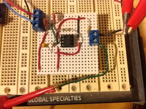
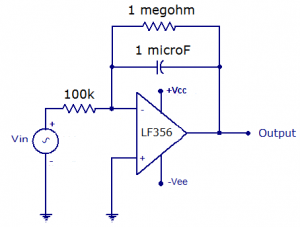
Something I've been wanting to do for a while was is to build a simple analog integrator. Here is my first attempt. I bread-boarded the circuit first to get it working then make it more permanent and stable by soldering the components onto a vero board. The picture below shows the result:

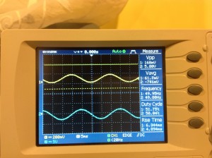
The three cables coming into the top left of the board are the +12, 0 and -12 volt power lines. The two cables coming out from the right-hand edge of the circuit board are the input and output lines (from the top) respectively. The input is fed from a function generator and the output fed to an oscilloscope. The figure below shows the result of the feeding a 50 Hz sine wave. Integration results in a cosine wave on the output. Note the two decoupling capacitors in the top left corner that despike the power lines. These are 0.1 microF capacitors.

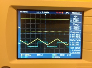
A final test shows the result of feeding in a square wave with the resulting triangle wave as output.

In the circuit I used a LF356 as the op amp which has a JFET input stage resulting in a very high input impedance and is typically used for precision high speed integrators. It is also quite cheap at about a dollar or less. The 1 megohm resistor across the integrator capacitor is there to avoid any unnecessary integration as a result of slight biases in the inputs when the input is supposed to be at zero.

There are a number of improvements that could be made to this circuit. The first is that any voltage bias as the inputs when both are set to zero should be removed by placing a potentiometer across the +voltage rail and the pot adjusted as appropriate. The second improvement is to add a reset button (mechanical or electronic) across the integrating capacity to reset the circuit when necessary.