How do I plot phase plots using Tellurium?

 Phase plots are a common way to visualize the dynamics of models where time courses are generated and one variable is plotted against the other. For example, consider the following model that can show oscillations:

  v1: $Xo -> S1; k1*Xo;
  v2:  S1 -> S2; k2*S1*S2^h/(10 + S2^h) + k3*S1;
  v3:  S2 -> ;   k4*S2;      

In this model S2 positively activates reaction v2 thus forming a positive feedback loop. The rate equation for v2 include a Hill like coefficient term, S2^h, which determines the strength of the positive feedback. The oscillations originate from an interaction between the positive feedback and a non-obvious negative feedback loop at S1 between v1 and v2.

Let us assign suitable parameter values to this model, run a simulation and plot S1 versus S2.

import tellurium as te
# Import pylab to access subplot plotting feature.
import pylab as plt

r = te.loada ('''
  v1: $Xo -> S1; k1*Xo;
  v2:  S1 -> S2; k2*S1*S2^h/(10 + S2^h) + k3*S1;
  v3:  S2 -> $w; k4*S2;      

  # Initialize
  h  = 2; # Hill coefficient
  k1 = 1; k2 = 2; Xo = 1;
  k3 = 0.02; k4 = 1;
  S1 = 6; S2 = 2
''')

m = r.simulate (0, 80, 500, ['S1', 'S2'])
r.plot()

Running this script by clicking the green button in the toolbar yields the following plot:

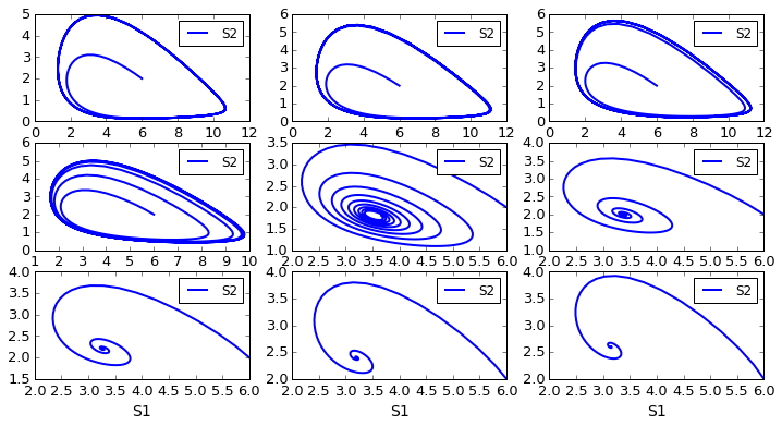
What if we'd like to investigate how the oscillations are affected by the parameters of the model. For example, how does the model behave when we change k1? One way to do this is to plot simulations at different k1 values onto the same plot. In this case, however, this will create a difficult to read graph. Instead, let us create a grid of subplots where each subplot represents a different simulation.

import tellurium as te
import pylab as plt

r = te.loada ('''
  v1: $Xo -> S1; k1*Xo;
  v2:  S1 -> S2; k2*S1*S2^h/(10 + S2^h) + k3*S1;
  v3:  S2 -> $w; k4*S2;      

  # Initialize
  h  = 2; # Hill coefficient
  k1 = 1; k2 = 2; Xo = 1;
  k3 = 0.02; k4 = 1;
  S1 = 6; S2 = 2
''')

plt.subplots(3,3,figsize=(12,6)) 
for i in range (9):
    r.reset()
    m = r.simulate (0, 80, 500, ['S1', 'S2'])
    plt.subplot (3,3,i+1)
    plt.plot (m[:,0], m[:,1], label="k1=" + str (r.k1))
    plt.legend()
    r.k1 = r.k1 + 0.2

Here we create a 3 by 3 subplot grid, start a loop that changes k1, and each time round the loop it plots the simulation onto one of the subplots. Running this script results in the following output